Abstract
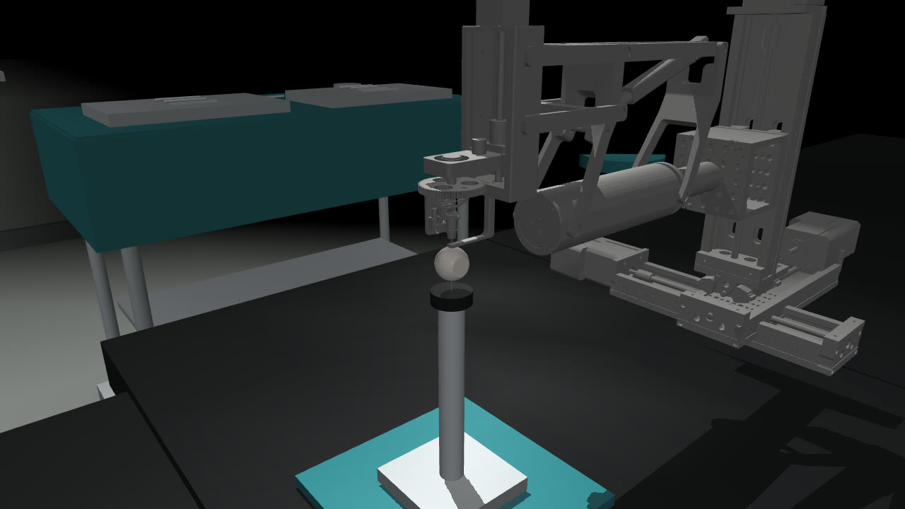
OmSR is a five-degree-of-freedom remote-centre-of-motion robot for vitreoretinal surgery, developed at Xi'an Jiaotong University and UCL.1,2 Published work covers its design, compliance control, vision-based automation and PPO-based tip navigation,1,2,21,22 but no simulation model of the robot is public. During a summer research internship at the UCL Hawkes Institute, I converted its CAD model into a kinematic MuJoCo simulator, whose tip positions lie within 0.85 mm of the published forward kinematics, and built a Gymnasium environment on it with four tasks: reaching a target in the vitreous cavity, peeling a rigid or a deformable membrane, and holding a 25-gauge needle at a target as a proxy for injection.
Four specification errors changed the environment after its validation scripts had passed, three of them exposed only by policy training: reach targets outside the eye, a released membrane whose fall drove the return of a single episode, a dimensionless sum of rewards, to −7,602, against about +20 for a successful one, a peel reward under which six of eight PPO policies scored 100 out of 100 while pushing the membrane 0.8 mm past the modelled retinal surface, and a stillness test that motion scaling made vacuous. At the default 1.5 mm tolerance and with the original stillness test, PPO learns the four tasks on 18 of 19 seeds and SAC learns the 3 tasks it was run on, on 9 of 9 seeds. Under the strict test that is now the default, PPO learned the injection only at a reduced initial policy standard deviation among the configurations tested. The evidence comes from a kinematic model without tissue contact, one to eight seeds per configuration, and success radii in millimetres.
1Introduction
In vitreoretinal surgery, instruments of 23 to 27 gauge, 0.64 to 0.41 mm in outer diameter, are introduced through trocar cannulas placed in the pars plana, 3.5 to 4 mm posterior to the limbus. Each instrument pivots about its sclerotomy, which leaves four degrees of freedom: two rotations about the port, insertion along the shaft and roll about its longitudinal axis. The surgeon operates under a microscope on structures such as the internal limiting membrane and epiretinal membranes on the retinal surface. OmSR enforces the pivot mechanically, and its design paper reports an end-effector motion error below 30 µm for each joint.1 The learning-based controllers for the eye in references 11 and 12 were trained from demonstrations collected on hardware; a simulator allows reinforcement learning and controlled evaluation without hardware in the loop.
Laparoscopic surgery has open reinforcement-learning environments: dVRL, SurRoL, LapGym and ORBIT-Surgical, built around the da Vinci Research Kit and similar robots.7–10 Inside the eye, learned control has been shown on other platforms, in both cases from demonstrations: navigating a tool to a retinal target11 and OCT-guided needle insertion into the cornea.12 Light-guide positioning19 and OCT registration for subretinal injection20 have been automated without learned control policies. On OmSR itself, the developers have added vision-based automatic control21 and TDN-PPO, which combines PPO with a tip-detection network to navigate the instrument tip to a target lesion.22 The closest simulation work trains reinforcement-learning policies for cataract incisions, in the anterior segment.15 I found no open reinforcement-learning environment for a posterior-segment robot and no public simulation model of OmSR. This environment provides both; I have not reproduced the training set-up of TDN-PPO.
Section 2 describes the conversion from CAD to MuJoCo and its validation against the published kinematics, Section 3 the interface and the tasks, Section 4 the PPO and SAC baselines, and Section 5 the specification errors. The environment was built during an eight-week research internship. The experiments in Sections 4 and 5 were run afterwards, in 106 runs on a rented cloud machine and 80 on a laptop. Every configuration has an identifier, such as P1 or I4, listed with its settings in Table A1, and all figures and tables are generated from the training logs and evaluation files.
2Kinematic model
2.1The robot
OmSR positions its instrument with five degrees of freedom:1 yaw \(\Phi\) over ±45° and pitch \(\Psi\) over 60° to 115°, both rotations about the RCM; insertion along the shaft, up to 30 mm; roll \(\theta\) of the instrument about its shaft, ±45°; and forceps opening, up to 12°. The code calls \(\Phi\) spin and \(\theta\) tool roll. The RCM is fixed by a double-parallelogram linkage rather than in software. The design paper reports an end-effector motion error below 30 µm for each joint. It reports RCM runout of 8.4 µm on average and 0.08 mm at most during pitching, and −10 µm on average and 0.083 mm at most during yaw.1 The second paper adds a double-loop admittance controller that regulates the instrument–tissue force to 40 mN, below a 60 mN threshold.2
Two simulated ranges differ from the published ones. Pitch is limited to 60° to 105°, the domain stated with Equation 3 of the design paper, whose text gives 60° to 115°. Roll is limited to ±90°, the joint limit in the CAD model, which is wider than the ±45° the paper states; none of the tasks requires roll, but policies are not prevented from using the wider range.
2.2From CAD to MuJoCo
The developers' CAD assembly was available as a Unity scene. I exported its joints and 63 meshes to a URDF with 16 links and 15 joints, computed masses and inertias from the mesh geometry, decimated the collision meshes from 300,000 to 27,000 faces and loaded the result into MuJoCo.3 The pitch mechanism is a closed kinematic loop, which URDF cannot represent, so its seven follower joints are coupled to the pitch joint with ratios of ±1.
A validation script checks each stage before the next is built on it. These scripts caught joint limits given in degrees where MuJoCo expected radians, a sign error on the insertion joint that displaced the tip by 66 mm opposite to the command, visual and collision meshes assigned to swapped geometry groups, which shifted the fitted pivot by 0.4 mm, and a tool-tip site that moved between the two forceps jaws from one build to the next.
2.3Locating the RCM
The entry point of the eye model, the depth limits and the RCM-error observation are all defined relative to the pivot, so I fitted it from the mechanism instead of taking it from a joint anchor in the CAD model. I posed the instrument at 42 configurations, a 6 × 7 grid over the pitch and yaw ranges, took the instrument axis in each, and solved for the point closest to all 42 lines. For lines through points \(a_i\) with unit directions \(u_i\), the point \(c\) that minimises the summed squared distance to the lines satisfies, with \(I\) the 3 × 3 identity,
The eye model was then placed so that its scleral entry point coincides with \(c\) to within 0.0005 mm, a numerical placement tolerance rather than a physical accuracy. Over 168 commanded poses, the 42 fitting configurations at four insertion depths, the instrument axis passes on average 0.23 mm and at most 0.40 mm from \(c\), and the residual grows towards both ends of the pitch range (Figure 2). Because these are the poses used for the fit, I also sampled 3,000 random poses over the full range of yaw, pitch, insertion and roll: the mean residual is 0.20 mm, the 95th percentile 0.34 mm and the maximum 0.41 mm. Joint positions are set exactly, so the residual is a property of the model geometry, not a control error. Part of it depends on roll: at 90° pitch it varies from 0.067 to 0.131 mm over the ±90° roll range. The instrument axis is taken through the roll-joint origin and the tip site, so this dependence means that the tip site lies slightly off the roll axis. The 0.41 mm maximum is five times the 0.08 mm maximum runout during pitching reported for the hardware.
I also compared the simulated kinematics with the forward-kinematics equations of the design paper at ten poses, two of them with insertion; Table A2 lists the poses, the frame alignment and the errors. Tip-position errors range from 0.20 to 0.85 mm. The direction error is 0.234° at every pose that varies a single coordinate, which matches a fixed tilt of the tool axis in the CAD model at the home pose; it is larger, up to 1.7°, where pitch and yaw are combined and the paper's direction vector departs from unit length. Four link lengths that can be matched to the paper's Table I agree to within 1.12 mm. I set no acceptance threshold in advance, and these errors exceed the 0.5 mm tolerance of Section 4.1.
2.4Fidelity
The internship brief called this model a digital twin. That term usually implies calibration against the physical system, which this model has not had, so I describe it as a CAD-derived kinematic simulator: it models and verifies the robot's geometry and motion, but not forces, tissue or the robot's controller. Table 1 compares it with the hardware and the clinical setting.
| Aspect | Simulator | Real robot or clinic |
|---|---|---|
| Geometry and kinematics | From CAD, tip within 0.85 mm of the published equations | Measured on the hardware |
| RCM deviation | 0.23 mm mean, 0.40 mm worst on the fitting grid | Runout 8.4 µm mean, 0.08 mm maximum during pitching; 0.083 mm maximum during yaw |
| Control | Joint positions set directly each step | 1 kHz joint loops, admittance control of tissue force |
| Tissue contact and force | None; grasping by proximity, depth limits as rules | Force regulated to 40 mN, threshold 60 mN |
| Precision | Task success radius 1.5 mm | Motion error below 30 µm per joint |
| Membrane | Rigid disc, or a 9 × 9 flex sheet released at 0.08 mm of stretch; grasp edge 0.51 mm in front of the retina | Internal limiting or epiretinal membrane on the retinal surface, peeled tangentially |
| Pitch and roll ranges | Pitch 60° to 105°, roll ±90° | Pitch 60° to 115°, roll ±45° |
| Observation | Exact state | Microscope image and OCT |
3The environment
3.1Interface
The environment implements the Gymnasium API.4 An action \(a \in [-1, 1]^5\) is scaled to per-step increments of at most 1° in pitch, 1° in yaw, 0.5 mm in insertion, 2° in roll and a quarter of the forceps range. The environment adds the increment to the current coordinates, clamps them to the simulated range and sets the yaw, pitch, insertion and roll joints, each of which differs from the corresponding RCM coordinate by a sign and an offset. The Cartesian gantry that carries the mechanism is fixed. The double-parallelogram linkage then constrains motion to rotations about the fitted entry point, subject to the geometric residual of Section 2.3, which reaches 0.41 mm. This property comes from the mechanism, which the environment preserves by never moving the gantry, and it holds only while joint positions are set directly.
The observation has nine robot values: pitch, yaw, insertion, roll, the tip position relative to the pivot, the RCM error and the forceps opening. Each task appends the goal position relative to the pivot and relative to the tip, where the goal is the target for reach and injection and the grasp edge for the peels. The peels add a grasp flag and the peel progress, which for the deformable sheet is the fraction of released pins; the injection adds the dwell counter and a delivery flag. All tasks share one per-step reward:
Here \(d_t\) is the remaining task distance, defined per task and phase in Appendix A.5; \(D\) is a normalising length of 20 mm for reach and 40 mm for the other tasks; \(\gamma = 0.99\) is the discount; \(e_t\) is the RCM error; and \(o_t\) is the depth past the task's limit. The limit is the retinal sphere for reach, the depth of the grasp edge for the peels and, for the injection, a point 2 mm short of the retinal sphere along the instrument axis. \(b_t\) is +1 on the first earned grasp in the deformable peel and +1 on delivery in the injection; the final injection reward also pays up to 0.05 per still step inside the target zone. The rigid peel has no bonus. The reward is dimensionless: every length in it is divided by \(D\), 1.5 mm or 1 mm, so per-step rewards and episode returns carry no unit.
The first term has the potential-based form \(\gamma\phi(s_t) - \phi(s_{t-1})\) with \(\phi = -2d/D\),6 but the potential is not set to zero at terminal states, so the policy-invariance result of that form does not hold exactly, and the other terms can change the optimal policy. The second is a dense distance penalty that saturates at \(d_t = D\). The third penalises the geometric residual of Section 2.3, which the policy can change only through pitch and roll. The fifth, the braking ramp, grows from 0 to 2 over the first millimetre past the depth limit. A task violation is insertion more than 1 mm past the depth limit, a membrane tear or the release of a fully peeled membrane. Terminal rewards are added to \(r_t\) on the last step: −20 for a task violation, +20 for success, and −100 for an RCM error above 1.5 mm, which cannot occur because the residual never exceeds 0.41 mm. Episodes are truncated at 300 steps, and the learning algorithms bootstrap truncated episodes from the value of the final state. Because violations start 1 mm past the limit, a reach policy can place the tip up to 1 mm beyond the retinal sphere without a violation, and a peel policy up to 0.49 mm beyond it.
3.2Tasks
Reach. Bring the tip within 1.5 mm of a target sampled uniformly over pitch 75° to 105°, yaw ±30° and depth from 15 mm to 1 mm in front of the retinal sphere, which gives depths of 15.0 to 18.9 mm. Rigid peel. A rigid disc 5 mm in diameter is centred 0.8 mm in front of the retinal sphere on a direction sampled over pitch 80° to 100° and yaw ±20°, which places its grasp edge 0.51 mm in front of the retina. The policy must close the forceps within 1.5 mm of the edge, pull the edge 3 mm along the line towards the entry point and withdraw until the tip is within 0.5 mm of the entry point. Deformable peel. The same sequence on a 9 × 9 flex sheet, 4.8 mm square, whose far edge is held by nine adhesion pins that release at 0.08 mm of stretch. It is the only task with dynamics: each control step integrates 25 physics steps of 2 ms with the robot held at its commanded pose. Appendix A.6 gives the mechanical parameters. Injection. A 25-gauge needle, 16 mm long, must reach a target sampled over pitch 78° to 102°, yaw ±28° and depth 12 to 16 mm, stay within 1.5 mm of it for ten consecutive steps while moving less than a stillness limit per step, and then withdraw. The kinematic tasks have no simulated time; the ten-step hold is meant to represent 0.5 s, which makes a step 50 ms, as in the deformable task, and the original 0.2 mm limit 4 mm/s. The released task applies the limit to the commanded motion, for the reasons given in Section 5.4.
3.3Verification
Each task has a scripted controller that acts through the same interface as the agent and succeeds in 20 of 20 test episodes. The scripted controllers demonstrate solvability on the tested resets, but do not rule out defects outside those trajectories. Each task also has a validation script that checks compliance with the Gymnasium API, tests every transition of the grasp and dwell state machines, applies random actions to confirm that the joints stay within range, and confirms that a fixed seed reproduces an episode exactly.
Every episode also logs, separately from success, the closest approach to the goal, the maximum depth past the membrane, whether the forceps grasped, the longest still run and the needle's speed inside the injection target. The three kinematic tasks need only forward kinematics, so they call mj_kinematics instead of mj_forward, which skips collision detection and the dynamics pipeline. Over 3,000 random steps per task, observations, rewards, termination flags and episode logs are bit-identical with and without this shortcut. Single-threaded on the laptop, an Apple M4 with MuJoCo 3.10 and Python 3.11, the shortcut raises throughput from 2,710 to 2,770 steps per second to 15,000 to 16,000, a factor of 5.5 to 5.8 depending on the task; across five timed repetitions of 3,000 steps the standard deviation is below 1% of the mean.
4Baselines
I trained PPO13 and SAC14 from Stable-Baselines3.5 PPO is on-policy, and the standard deviation σ of its Gaussian policy is a learned parameter per action dimension, independent of the state and initialised at 1 unless stated otherwise. SAC is off-policy, learns from a replay buffer, and its policy network outputs a state-dependent standard deviation. Hyperparameters are in Appendix A.1.
Four outcome measures appear below and are kept distinct. The training success rate is the fraction of the last 100 training episodes that succeed, counting only episodes that start from the reset state. The evaluation score is the number of successes in 100 evaluation episodes with fixed seeds, using the deterministic mean action of the final weights. A seed counts as having learned the task if its evaluation score is at least 90. Steps to 90% is the first training step at which the training success rate reaches 90%, whether or not that seed later passes evaluation.
With the lenient stillness test, every PPO and SAC seed scores at least 87 out of 100 and all but one at least 95. PPO learns the four tasks on 18 of 19 seeds and SAC learns reach, rigid peel and injection on 9 of 9. Under the strict stillness test, the released default, PPO learns the injection on 0 of 8 seeds. Learned PPO peel policies, rigid and deformable, finish in 58 steps and SAC rigid-peel policies in 58.4 to 59.5, inserting at the 0.5 mm per-step limit on the approach, while the scripted controller takes 82.8 steps on the rigid peel. SAC reached 90% sooner on the injection, at 205,000 steps against 313,000, and later on reach, at 113,000 against 81,000; with three to eight seeds per configuration I do not treat these differences as established. In evaluation, the lenient-injection policies end 7 of 800 PPO episodes and 1 of 300 SAC episodes in a depth violation; no other baseline policy has a violation.
Outcomes for a given seed did not always transfer between machines. In configuration P2, the rigid peel run on the laptop with eight seeds, seed 1 never learned: it brought the open forceps to 0.28 mm from the membrane edge and never closed them. The same seed and hyperparameters learned the task on the cloud machine in P1. Injection seed 2 scored 73 on the laptop in I2 and 99 on the cloud in I1. The machines share MuJoCo 3.10, Gymnasium 1.3 and Stable-Baselines3 2.9 but differ in PyTorch, 2.13.0 against 2.14.1, in NumPy, 2.4.6 against 2.1.2, and in thread counts; which difference is responsible is not established. Figure 4 shows every run.
4.1Sub-millimetre tolerances
The 1.5 mm success radius is 50 times the 30 µm per-joint motion error reported for the hardware. The two measure different things, a task tolerance and a positioning error, but the ratio shows how far the task specification is from the robot's precision. I retrained reach at success radii of 1.5, 0.5, 0.1 and 0.03 mm, configurations R1 to R4, three seeds each for 1 million steps (Figure 5). All seeds learn at 1.5 and 0.5 mm. At 0.1 mm the seeds score 0, 4 and 4 out of 100, with closest approaches of 1.52, 0.93 and 0.96 mm, and at 0.03 mm all score 0. Episodes end when the tip enters the tolerance ball, so the closest approach of the successful policies, 1.27 mm at 1.5 mm and 0.30 mm at 0.5 mm, is set by termination and cannot be compared with that of the failed policies.
At 0.1 mm the training success rate over the last 2,000 episodes is 4 to 16%, but σ stays between 0.89 and 0.97, and the deterministic policy stops 0.93 to 1.52 mm from the target. Three untested explanations are compatible with this: the entropy bonus of 0.005 opposes the decay of σ; sampled actions are clipped to [−1, 1], which at σ ≈ 0.9 shifts the mean executed action away from the policy mean; and the last millimetre carries little return, since with \(D = 20\) mm closing the final 0.9 mm changes the shaped terms by about 0.09 while the +20 bonus is collected in the noisy episodes that succeed. Remedies such as motion scaling near the target, hindsight experience replay23 or a logarithmic distance term are also untested. The tasks as released are specified at millimetre scale. TDN-PPO reports micrometre-scale accuracy on the same robot,22 with a set-up I have not compared with this one.
5Specification errors exposed by training
Four findings changed the environment after all of its validation scripts had passed. One came from checking the code against the eye geometry; the other three appeared only in training. Because policy optimisation visits states that the validation scripts do not enumerate, the environment now logs penetration depth, closest approach, grasp state, longest still run and in-zone needle speed for every episode.
5.1Two bugs the validation scripts missed
The first came from comparing the reach task's target depths with the geometry of the eye. Targets were sampled 15 to 22 mm past the entry point, but along the sampled directions the retinal sphere lies only 16.9 to 20.0 mm away, and 424 of 1,000 sampled targets lay outside the eye. No term penalised these targets: insertion to the 30 mm joint limit, 10 to 13 mm beyond the retinal sphere, incurred no penalty. Policies trained on this version, configuration R7, scored 100 out of 100. Targets are now sampled at least 1 mm in front of the retina, and insertion more than 1 mm beyond it is a task violation.
The second appeared only because training failed. In the deformable peel as committed at the end of the internship, configuration F4, a policy that completed the peel and then opened the forceps released a sheet that no pin held. The eye model has no contact surface, so the sheet fell under the applied weight for the rest of the episode, and the remaining task distance, which is measured to the falling sheet, grew without a cap. The progress term turned this into episode returns as low as −7,602, where a successful episode returns about +20, most of it the success bonus. For scale, free fall over a whole 300-step episode of 15 s covers ½gt2 = 1.1 km; this is an idealised bound, not a logged trajectory. In the one run that completed, 266 of its 4,250 episodes returned less than −60 and the policy never learned the task; a second seed, stopped after 565 episodes, had 113 such episodes. Releasing a fully peeled membrane is now a task violation. After the fix, in F1, 11 of 30,942 episodes across three seeds returned less than −60, none less than −67, and all three seeds learned.
5.2Reward exploitation in the rigid peel
An early version of the rigid peel, configuration P5, counted any displacement of the grasped edge as progress, regardless of direction. All eight seeds score 100 out of 100, and six of them complete the "peel" by pushing the membrane 1.33 to 1.36 mm past its initial position, averaged over evaluation episodes. The membrane edge rests 0.51 mm in front of the retina, so these trajectories end 0.82 to 0.85 mm beyond the modelled retinal surface. The other two seeds peel outward as intended (Figure 6). Which strategy a run learns varies with the seed, and the success rate does not distinguish them. Specification gaming of this kind is well documented in reinforcement learning.16 Here the trajectory crosses the modelled retinal boundary; its physical consequences were not simulated, and the success criterion does not detect it.
The corrected reward counts only movement along the pull direction. The environment also reports penetration depth, closest approach and the other per-episode measurements of Section 3.3 alongside success, so a policy that succeeds through the wrong behaviour can be detected without inspecting its rollouts.
5.3Reconstructed reward ablations
The task versions in Table 3 replace five earlier versions that were specified in written notes at the time; their code was not retained. I reimplemented each from the notes and retrained it, three seeds each, against the same task with the fix applied. Because the old versions are reconstructions and three seeds per side cannot resolve small effects, these comparisons are indicative only.
Only the first row reaches p < 0.05, and after Holm correction over the five rows its p-value is 0.12. With a 20 mm normaliser on a task that spans about 40 mm, the dense distance term saturates throughout the approach, so its gradient there is zero and only the potential-based progress term points towards the membrane. None of the three runs ever grasped, and their mean closest approach was 9.7 mm; why the progress term alone was insufficient was not measured. Row 2 is a control I added, not the version in the notes. That version, P10, which switched the distance at each phase and used the 20 mm normaliser, learned the task on the one seed I tried. To separate the phase switch from the saturation, row 2 uses the 40 mm normaliser on both sides. In a scripted rollout under this reward, the step that completes the grasp is charged −0.16 and the step that completes the peel −0.77, against a mean of −0.002 for the other steps. Two of the three runs stopped 2.13 and 2.15 mm from the edge, 0.6 mm outside the grasp radius, which is consistent with the cost at the grasp boundary but does not establish it as the cause.
Row 3, a rule that tears the deformable membrane when it is pulled faster than 0.35 mm per step, is the only variant that produced partial learning, with scores of 38, 62 and 0, which makes it a candidate for a harder released task. A hard −100 penalty without the braking ramp did not prevent learning, contrary to the conclusion recorded at the time, but it doubled the training steps needed to reach 90%, from 265,000 to 505,000. Row 5 also changes the penalty from −20 to −100, so it cannot attribute the slowdown to either change.
5.4Exploration noise and the injection hold
The injection's original stillness test required ten consecutive steps within 1.5 mm of the target at less than 0.2 mm per step. Four rewards failed on it with PPO at σ = 1, each on three seeds: the bare requirement, a per-step payment for stillness, a stillness payment that increases towards the target centre, and that payment combined with episodes that start already delivered, configurations I11 and I8 to I10. Under the per-step payment, the deterministic policies complete the hold in 51, 88 and 83% of evaluation episodes but never withdraw. The reward that was learned, I1, adds motion scaling, which multiplies actions by a factor falling linearly from 1 at 5 mm from the target to 0.25 at 1.25 mm and below.
With motion scaling the stillness test is vacuous. Inside the 1.5 mm target zone the factor is 0.25 to 0.3, so every possible step moves the needle less than 0.2 mm, and the learned policies move it 0.095 to 0.105 mm per step during the "hold", about 2 mm/s at a 50 ms step. When the test is instead applied to the commanded motion before scaling, which tightens the limit on the actual motion to 0.05 to 0.06 mm inside the zone, the same reward, starting states and motion scaling learn on 0 of 8 seeds at σ = 1, configuration I4, and on 3 of 8 at σ = 0.25, I5 (Figure 8). Five of the eight seeds in I5 fail mainly before the hold: they enter the target zone in only 3 to 40 of 100 evaluation episodes, with mean closest approaches of 2.25 to 2.99 mm.
The training data are consistent with exploration noise limiting the hold. With the needle at the target centre and σ = 1, 6% of sampled actions move it less than 0.2 mm. If the policy mean is zero and steps are independent, ten consecutive still steps then occur with probability 6.6 × 10⁻¹³, and in the last 2,000 training episodes at σ = 1 and 0.7 no hold was completed, so the value function never observed the delivery bonus. The same estimate orders the settings correctly for σ ≥ 0.5, where training completed holds in 0, 0 and 0.3% of episodes, but it is not a quantitative prediction: at σ = 0.35 it gives 0.006 against a training hold rate of 46%, and at σ = 0.15 it gives 0.89 against 24%, because a trained policy's mean is not zero and its steps are not independent.
With the bare reward, configuration I6, lowering the initial σ made the hold learnable without stillness payments, delivered starts or motion scaling. At σ ≥ 0.5 no seed completes a single injection in evaluation, 0 of 24. At σ = 0.35 seven of eight seeds succeed in at least one evaluation episode and two in at least 90; at σ = 0.25 all eight succeed at least once and four in at least 90; at σ = 0.15 one of eight learns. The deterministic policies trained at σ = 1, 0.7 and 0.5 complete the hold in 10, 37 and 49% of evaluation episodes on average but never withdraw. At σ = 1 this happens although no training episode in the last 2,000 completed a hold; how the mean policy comes to hold still is an open question. SAC on the bare reward, I7, learns on two of three seeds, which hold at 0.09 mm per step; the third never holds and raises the SAC mean in Figure 8 to 0.17 mm. SAC differs from PPO in its replay buffer, network size, entropy tuning and reward normalisation as well as in its state-dependent noise, so this comparison does not isolate the noise.
Within the tested configurations, reliable learning of the hold occurred only at lower initial σ. The sensitivity of PPO to its initial σ is known.17 PPO without the entropy bonus, PPO with state-dependent exploration18 and a lower σ for the shaped rewards were not tested, so the runs do not show that shaping is irrelevant.
Lowering σ also changed the rigid peel. At σ = 0.25, configuration P4, three of five seeds learned instead of five of five in P1, and the seeds that learned needed about three times as many steps to reach 90%, 894,000 against 301,000 on average. One of the two that failed reached a 90% training success rate at 1.06 million steps, fell to 22% over its last 2,000 episodes and scored 0 in evaluation. The released injection task applies the stillness test to the commanded motion, and the lenient version remains available by name to reproduce the earlier results. Results on the injection should be reported with the initial σ.
6Limitations and next steps
The simulator is kinematic and CAD-derived, without calibration against the hardware. Joint positions are set rather than driven, there is no instrument–tissue contact, and the retina is a depth rule rather than a surface. That rule is a sphere fitted to the posterior eye wall, which does not describe the wall elsewhere; the entry point itself lies inside the sphere. Violations begin 1 mm past each depth limit, so policies may place the tip up to 1 mm beyond the retina in reach and 0.49 mm beyond it in the peels.
Several task details differ from clinical practice. The membrane edge sits 0.51 mm in front of the retina instead of on it. Peel progress is measured along the line to the entry point, 7° to 29° from the retinal normal, which rewards traction away from the retina, whereas clinical membrane peeling is tangential. The forceps grasp anywhere within 1.5 mm of the edge, and the learned policies close them 1.2 mm short of it. The injection target is a point 12 to 16 mm deep in the vitreous, reached with a 25-gauge needle; clinical intravitreal injections are given by hand with finer needles, and the procedures that need a robot, such as subretinal injection, need holds well below 0.1 mm.
The released tasks do not separate PPO, SAC and the scripted controllers, except the strict injection, which PPO at σ = 1 does not learn and SAC has not been run on. Policies observe the exact state rather than a microscope image and are evaluated on the target distribution they were trained on. Learnability also depends on normalisation: reach without observation and reward normalisation, configuration R6, scores 10, 7 and 0 out of 100, and the observation mixes radians and metres. Each configuration has one to eight seeds, results are reported per seed without confidence intervals, and individual seeds did not always give the same outcome on the two machines.
The next step is graded task variants that separate methods, evaluated with PPO, SAC and the scripted controllers on at least five seeds each. Candidates are the tearing rule of Section 5.3, a force limit derived from the 60 mN threshold of the compliance paper, sub-millimetre reach with motion scaling, and held-out target regions. The task geometry should place the membrane on the retinal surface, measure peel progress tangentially and put the violation at the retina. On the injection, a factorial study of σ and reward shaping would test the conclusion of Section 5.4 directly. Longer-term work is to drive the joints through a model of the closed pitch loop, to add contact and a tissue model, and to replace the exact state with the microscope image or simulated OCT. A prototype of the closed loop enforces the pitch linkage with equality constraints instead of setting the follower joints; while its pitch joint was servoed from −30° to +50°, the free followers stayed within 0.042° of the ±1 coupling law. Measured hardware parameters, such as the reducer ratios and motor masses missing from the CAD model, would allow the dynamics to be identified against the real robot.
ADetails
A.1Training settings
PPO: Stable-Baselines3 2.9, two hidden layers of 128 units, 8 parallel environments, 512 steps per environment per update, minibatch 1,024, 10 epochs, learning rate 3·10−4, entropy coefficient 0.005, clipping 0.2, GAE λ 0.95, discount 0.99, observations and rewards normalised with running statistics. SAC: the library defaults of two layers of 256 units, a replay buffer of one million transitions, batch 256 and automatic entropy tuning; one environment; discount 0.99; observations normalised, rewards not. Budgets are in Table A1. Every evaluation uses the weights at the end of training; no checkpoint was selected.
A.2Compute
The validation scripts and 80 training runs used a laptop with an Apple M4 and ten CPU cores: 12 single-seed pilot runs, 58 study runs, 7 deformable-peel runs that predate the fix of Section 5.1, and 3 reach runs repeated after the target fix. Of these, Table A1 lists the runs the text reports. R7 comes from the internship. The 106 cloud runs used a 61-CPU share of a rented AMD EPYC 7B13 machine with two RTX 3070 GPUs for 3 hours 45 minutes, at a cost of $1.48. Three setup problems were fixed before those runs and the affected runs discarded: CPU jobs opening GPU contexts, numerical libraries starting 128 threads per job, and the full mj_forward step described in Section 3.3. Results are compared only between runs on the same machine, because the same seed did not always give the same outcome on both.
A.3Reproducing the results
The project is still in development: the code repository, HakimElAyoubi/Omsr-digital-twin on GitHub, is private, and the training logs and evaluation files are not yet publicly available. The procedure below applies once they are released. The environment, validation scripts, training and analysis code are in that repository; the results were produced at commit c8d277d with MuJoCo 3.10.0, Gymnasium 1.3.0, Stable-Baselines3 2.9.0 and Python 3.11, and PyTorch 2.13.0 on the laptop and 2.14.1 on the cloud machine. One run is trained and evaluated with scripts/train_ppo.py --task TASK --variant VARIANT --seed S, adding --algo sac, --log-std-init or --tol-mm as Table A1 requires; scripts/run_ablations.py runs whole sets, and scripts/analyze_study.py summarises them. The fast-path check of Section 3.3 is scripts/check_fast_kinematics.py. Every figure on this page is drawn from media/results.js, which build/export_results.py generates from the training logs and evaluation files; both are published with the source of this post.
A.4Experiment registry and kinematic validation
Table A1 lists every configuration the text reports, and Table A2 the forward-kinematics comparison of Section 2.3. The four link lengths compared with Table I of the design paper are the beam l2 + l7, 205.00 mm in both; the mid link l9, 76.71 mm against 75.70 mm, where the paper's own relation l5 + l6 = l9 gives 76.70 mm; the push-rod anchor l11, 108.94 mm against 109.50 mm; and the end-effector offset l6 + l9, 137.78 mm against 138.90 mm.
| ID | Task and version | Success criterion | Starts | Algorithm, σ₀ | Steps | Machine | Seeds | Reported in |
|---|---|---|---|---|---|---|---|---|
| R1 | Reach, final | 1.5 mm | none | PPO, 1 | 1M | C | 3 | Table 2, Fig. 4, 5 |
| R2 | Reach, final | 0.5 mm | none | PPO, 1 | 1M | C | 3 | Fig. 5 |
| R3 | Reach, final | 0.1 mm | none | PPO, 1 | 1M | C | 3 | Fig. 5, §4.1 |
| R4 | Reach, final | 0.03 mm | none | PPO, 1 | 1M | C | 3 | Fig. 5 |
| R5 | Reach, final | 1.5 mm | none | SAC | 400k | C | 3 | Table 2, Fig. 4 |
| R6 | Reach, final, no normalisation | 1.5 mm | none | PPO, 1 | 400k | L | 3 | §6 |
| R7 | Reach, targets outside the eye | 1.5 mm | none | PPO, 1 | 400k | L | 3 | §5.1 |
| P1 | Rigid peel, final | peel and withdraw | none | PPO, 1 | 1.5M | C | 5 | Table 2, Fig. 4, §5.4 |
| P2 | Rigid peel, final | peel and withdraw | none | PPO, 1 | 1.5M | L | 8 | §4, Table 3 |
| P3 | Rigid peel, final | peel and withdraw | none | SAC | 1M | C | 3 | Table 2, Fig. 4 |
| P4 | Rigid peel, final | peel and withdraw | none | PPO, 0.25 | 1.5M | C | 5 | §5.4 |
| P5 | Rigid peel, any displacement counts | peel only | none | PPO, 1 | 1.5M | L | 8 | §5.2, Fig. 6, 7 |
| P6 | Rigid peel, directional, −100 cliff | peel only | none | PPO, 1 | 1.5M | L | 3 | Fig. 6, 7, Table 3 |
| P7 | Rigid peel, directional, braking ramp | peel only | none | PPO, 1 | 1.5M | L | 3 | Table 3 |
| P8 | Rigid peel, phase switch, D 40 mm | peel and withdraw | none | PPO, 1 | 1.5M | L | 3 | Table 3 |
| P9 | Rigid peel, continuous distance, D 20 mm | peel and withdraw | none | PPO, 1 | 1.5M | L | 3 | Table 3 |
| P10 | Rigid peel, phase switch, D 20 mm | peel and withdraw | none | PPO, 1 | 1.5M | L | 1 | §5.3 |
| F1 | Deformable peel, final | peel and withdraw | 50% grasped | PPO, 1 | 600k | L | 3 | Table 2, 3, Fig. 4 |
| F2 | Deformable peel, pull-rate tearing | peel and withdraw | 50% grasped | PPO, 1 | 600k | L | 3 | Table 3 |
| F3 | Deformable peel, no grasp bonus | peel and withdraw | none | PPO, 1 | 600k | L | 3 | Table 3 |
| F4 | Deformable peel, before the release fix | peel and withdraw | 50% grasped | PPO, 1 | 600k | L | 1 + 1 stopped | §5.1 |
| I1 | Injection, final | lenient | 50% delivered | PPO, 1 | 600k | C | 8 | Table 2, Fig. 4, 8 |
| I2 | Injection, final | lenient | 50% delivered | PPO, 1 | 600k | L | 3 | §4 |
| I3 | Injection, final | lenient | 50% delivered | SAC | 600k | C | 3 | Table 2, Fig. 4 |
| I4 | Injection, final | strict | 50% delivered | PPO, 1 | 600k | C | 8 | Table 2, Fig. 8 |
| I5 | Injection, final | strict | 50% delivered | PPO, 0.25 | 600k | C | 8 | Fig. 8 |
| I6 | Injection, bare | lenient | none | PPO, 1 to 0.15 | 600k | C | 8 per σ₀ | Fig. 8 |
| I7 | Injection, bare | lenient | none | SAC | 600k | C | 3 | Fig. 8 |
| I8 | Injection, stillness payment | lenient | none | PPO, 1 | 600k | L | 3 | §5.4 |
| I9 | Injection, centre-weighted payment | lenient | none | PPO, 1 | 600k | L | 3 | §5.4 |
| I10 | Injection, centre-weighted payment | lenient | 50% delivered | PPO, 1 | 600k | L | 3 | §5.4 |
| I11 | Injection, bare | lenient | none | PPO, 1 | 600k | L | 3 | §5.4 |
| Pose | Ψ (°) | Φ (°) | Insertion (mm) | Direction error (°) | Tip error (mm) |
|---|---|---|---|---|---|
| Home | 90 | 0 | 0 | 0.234 | 0.41 |
| Yaw +20° | 90 | 20 | 0 | 0.234 | 0.43 |
| Yaw −30° | 90 | −30 | 0 | 0.234 | 0.42 |
| Pitch 75° | 75 | 0 | 0 | 0.234 | 0.20 |
| Pitch 105° | 105 | 0 | 0 | 0.234 | 0.62 |
| Insertion 20 mm | 90 | 0 | 20 | 0.234 | 0.41 |
| Combined | 80 | 25 | 0 | 0.432 | 0.41 |
| Combined | 100 | −20 | 0 | 0.338 | 0.59 |
| Combined, inserted | 70 | 40 | 10 | 1.729 | 0.85 |
| Combined | 95 | −45 | 0 | 0.246 | 0.52 |
A.5Reward and reset specification
Here \(z\) is the insertion depth past the pivot, and \(z_{\text{out}} = 0.5\) mm is the depth at which the instrument counts as withdrawn. Reach: \(d = \lVert x_{\text{tip}} - x_{\text{target}} \rVert\). Rigid peel: before the grasp, \(d = \lVert x_{\text{tip}} - x_{\text{edge}} \rVert + L + (z_{\text{edge}} - z_{\text{out}})\) with \(L = 3\) mm; while peeling, \(d = (L - p) + \max(z - z_{\text{out}}, 0)\), where \(p\) is the largest displacement of the grasped edge along the pull direction so far; after the peel, \(d = \max(z - z_{\text{out}}, 0)\). Deformable peel: the same, with \(x_{\text{edge}}\) the grasp vertex and \(L - p\) replaced by \((1 - f)\cdot 4.8\) mm, where \(f\) is the fraction of released pins. Injection: before delivery, \(d = \lVert x_{\text{tip}} - x_{\text{target}} \rVert + (1 - k/10)\cdot 2\ \text{mm} + (z_{\text{target}} - z_{\text{out}})\), where \(k\) is the current count of consecutive still steps; after delivery, \(d = \max(z - z_{\text{out}}, 0)\).
The stillness payment of the final injection reward is, on each step inside the 1.5 mm zone, \(0.05 \cdot \max(0, 1 - \Delta/\tau) \cdot (1 - e/1.5\ \text{mm})\), where \(\Delta\) is the tip displacement on that step, \(\tau\) the stillness limit and \(e\) the distance to the target; the per-step payment of I8 omits the last factor. \(\tau\) is 0.2 mm under the lenient test and 0.2 mm times the motion-scaling factor under the strict test.
Grasped starts, in half of the F1, F2 and F4 training episodes, place the tool on the line from the pivot to the grasp vertex, 0.4 mm short of the vertex, with the forceps closed and the grasp constraint active. Delivered starts, in half of the I1 to I5 and I10 training episodes, place the needle tip at the sampled target with the hold complete, so only withdrawal remains. Neither kind of start pays the grasp or delivery bonus, and evaluation never uses them.
A.6Deformable membrane
The membrane is a MuJoCo flex grid of 9 × 9 vertices at 0.6 mm spacing, a 4.8 mm square, with a total mass of 0.05 g and a vertex radius of 0.15 mm. Its edges are equality constraints with solver reference time 2 ms and damping ratio 1, plus an edge damping of 0.002; self-collision is on and contact with the eye is off. The nine vertices of the far row are held by connect constraints to fixed anchors, with time constant 2 ms, each released when its vertex moves more than 0.08 mm from its anchor. The grasp is a connect constraint between the forceps tip and the middle vertex of the near row, with time constant 1 ms, switched on when the closed forceps are within 1.5 mm of that vertex. Scene gravity is zero; once the sheet is grasped or a pin has released, each vertex receives its weight at 9.81 m/s² as an applied force. The physics step is 2 ms with MuJoCo's Euler integrator and Newton solver, at most 100 iterations, and after every physics step the robot's joints are reset to their commanded positions with zero velocity. A grasp strain above 1 mm tears the membrane, a task violation.
References
- Wang, Zhang, Li, Zhang, Stoyanov and Stilli (2022). A 5-DOFs robot for posterior segment eye microsurgery. IEEE Robotics and Automation Letters.
- Wang, Zhang, Stoyanov, Zhang and Stilli (2023). Vision-and-force-based compliance control for a posterior segment ophthalmic surgical robot. IEEE Robotics and Automation Letters. doi:10.1109/LRA.2023.3313065.
- Todorov, Erez and Tassa (2012). MuJoCo: a physics engine for model-based control. IROS.
- Towers et al. (2024). Gymnasium: a standard interface for reinforcement learning environments. arXiv:2407.17032.
- Raffin et al. (2021). Stable-Baselines3: reliable reinforcement learning implementations. JMLR 22.
- Ng, Harada and Russell (1999). Policy invariance under reward transformations. ICML.
- Richter, Orosco and Yip (2019). Open-sourced reinforcement learning environments for surgical robotics. arXiv:1903.02090.
- Xu et al. (2021). SurRoL: an open-source reinforcement learning centered and dVRK compatible platform for surgical robot learning. IROS.
- Scheikl et al. (2023). LapGym: an open source framework for reinforcement learning in robot-assisted laparoscopic surgery. JMLR 24.
- Yu et al. (2024). ORBIT-Surgical: an open-simulation framework for learning surgical augmented dexterity. ICRA.
- Kim et al. (2020). Autonomously navigating a surgical tool inside the eye by learning from demonstration. ICRA.
- Keller et al. (2020). Optical coherence tomography-guided robotic ophthalmic microsurgery via reinforcement learning from demonstration. IEEE Transactions on Robotics.
- Schulman, Wolski, Dhariwal, Radford and Klimov (2017). Proximal policy optimization algorithms. arXiv:1707.06347.
- Haarnoja, Zhou, Abbeel and Levine (2018). Soft actor-critic: off-policy maximum entropy deep reinforcement learning with a stochastic actor. ICML.
- Gomaa et al. (2023). Toward a surgeon-in-the-loop ophthalmic robotic apprentice using reinforcement and imitation learning. arXiv:2311.17693.
- Krakovna et al. (2020). Specification gaming: the flip side of AI ingenuity. DeepMind blog.
- Andrychowicz et al. (2021). What matters for on-policy deep actor-critic methods? A large-scale study. ICLR.
- Raffin, Kober and Stulp (2021). Smooth exploration for robotic reinforcement learning. CoRL.
- Koyama, Marinho, Mitsuishi and Harada (2022). Autonomous coordinated control of the light guide for positioning in vitreoretinal surgery. IEEE Transactions on Medical Robotics and Bionics 4(1).
- Mach et al. (2022). OCT-guided robotic subretinal needle injections: a deep learning-based registration approach. IEEE BIBM.
- Wang, Zhang, Bano, Stoyanov, Zhang and Stilli (2025). Vision-based automatic control of a surgical robot for posterior segment ophthalmic surgery. IEEE Transactions on Automation Science and Engineering 22. doi:10.1109/TASE.2024.3438452.
- Wang, Zhang, Bano, Stoyanov, Liang and Stilli (2026). TDN-PPO: an automatic control framework of a surgical robot for posterior segment ophthalmic surgery. IEEE Transactions on Automation Science and Engineering 23. doi:10.1109/TASE.2026.3671981.
- Andrychowicz et al. (2017). Hindsight experience replay. NeurIPS.