Abstract
A connectome is the complete wiring diagram of a nervous system: every neuron, and every connection between neurons, traced from electron microscope images. In September 2026 the first complete connectome of an adult male fruit fly was published. It records which neurons connect, how many synapses join them and whether each neuron excites or inhibits its targets. It does not record how strong each connection is in the living animal.
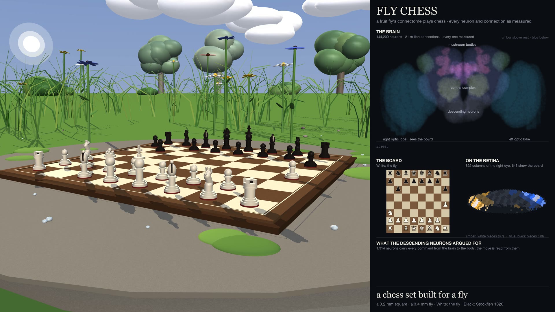
That gap allows a clean experiment. If the wiring is kept exactly as measured and only the connection strengths are learned, can the fly's brain be trained on a task it never evolved for, and which of its circuits does the trained network rely on? I used chess as the task. I simulated the 144,209 neurons of the fly's brain, showed it chess positions through the photoreceptors of its right eye, read its chosen move from the 1,314 descending neurons that normally carry commands from the brain to the body, and trained the connection strengths on 4.3 million positions from human games.
Before any filtering, the trained network's first choice is a legal move 80% of the time and matches the move the human played 23% of the time. In matches it beats a random mover and loses almost every game to the weakest Stockfish setting. Switching off groups of neurons costs most for the visual pathway and the descending neurons, and nothing measurable for the mushroom body (the fly's centre for learning and memory) or the central complex (which supports navigation); the way the move is read out, however, makes small and null effects hard to interpret. These results are preliminary. No rewired, dense or non-connectome baseline has been trained, the positions used for the silencing experiments overlap the training data, and match scores varied between repeated runs. A final phase in which the network learned from its own games increased draws and reduced wins, for reasons not yet established.
1Introduction
A real fruit fly cannot play chess. Each compound eye has fewer than a thousand facets, most of what the fly learns is simple association, and nothing it does requires planning several steps ahead. The question here is narrower: what a network with this fly's wiring can learn when it is trained, which is a different thing from what the fly itself can do.
The connectome used here, released by Janelia, the Cambridge connectomics group and Google Research, covers the male fly's brain and nerve cord.1 Synapse counts are a reasonable proxy for connection strength but not the same thing: receptor densities, where a synapse sits on the dendrite and other properties invisible to electron microscopy all change how much one neuron influences another. A mixing desk is a fair picture. Every cable has been traced, and none of the volume settings were written down.
Chess suits the question for practical reasons. The input is a static image, the output is a discrete choice with an exact legality rule, millions of labelled positions are freely available, and strong engines provide a fixed yardstick. This post describes one trained network, and is explicit about what can and cannot yet be concluded from it.
2Method
Sections 2 and 3 use no equations. The model, encoding and training details are in Appendix A.
2.1The digital fly
The model contains the 144,209 traced neurons on the brain side of the neck, joined by 21.27 million connections that carry 99.4 million synapses. Each neuron's sign comes from its predicted transmitter. Acetylcholine neurons excite their targets, and GABA and glutamate neurons inhibit them. Dopamine, serotonin and octopamine neurons act through slower modulatory signalling that this kind of model cannot represent, so their outgoing connections are removed; their own activity is still computed.
Each simulated neuron holds one number, its rate, which starts at zero for every move. Every 5 ms tick, that rate moves a quarter of the way toward a saturating function of the neuron's summed input, which gives the network a 20 ms time constant. One move is 24 ticks, or 120 ms of simulated time.
I set the one free scale parameter of the model using two checks taken from fly experiments, so these checks calibrate the model rather than independently validate it. Driving the 187 sugar-sensing taste neurons should push MN9, the motor neuron that starts feeding, above rest. It did, by 1.1% of the network's peak response, which ranks MN9 in the top 2% of all neurons and 4.8 standard deviations above twenty control runs. The controls were meant to be random sensory sets of the same size, but the pool of other labellar taste neurons has only 58 members, so ten of the twenty controls are the same 58 neurons; the other ten are random sets of 187 mechanosensory neurons. Light on the right eye should drive the right eye's lamina and leave the left eye's quiet: the mean activity of the right L1 and L2 cells rose to 0.216 of the network's peak response, against 0.0002 on the left.
2.2Showing it the board
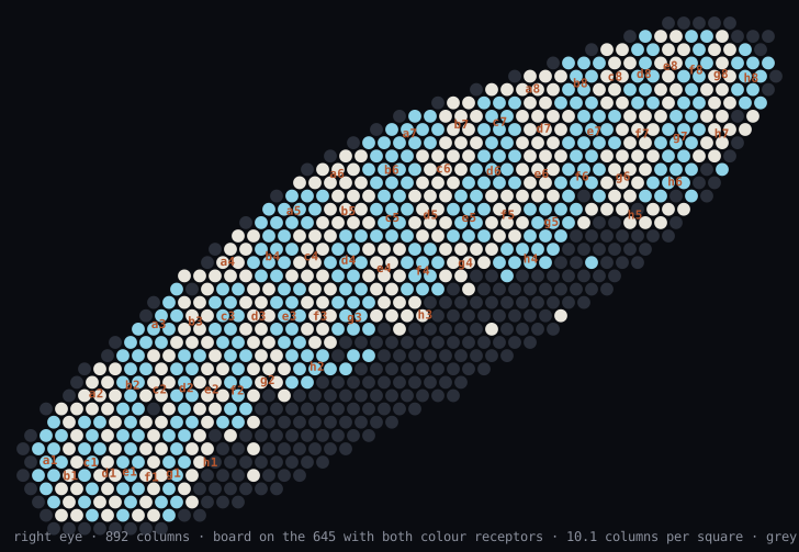
A fly's eye is a hexagonal grid of columns, each looking at one point in space, and the connectome assigns most visual neurons to a column. That makes the right eye usable as a screen. Of its 892 columns, the 645 that contain both colour-sensitive photoreceptor types became the board, about ten columns per square.
Ten columns cannot resolve the shape of a knight, so pieces are encoded by colour. The R7 and R8 photoreceptors respond to different wavelengths, and each of the thirteen states a square can be in (empty, or one of six piece types in either colour) is a pair of intensity levels on those two channels (Figure 3). The broadband R1–R6 receptors carry one more piece of information: a uniform brightness shift when Black is to move.
I then measured how much of the board survives each stage of the untrained network. I ran the model on 8,192 random placements of pieces and 1,024 positions from random play, and fit a linear decoder that recovers every square from each region's activity (Figure 4); the figure reports held-out random placements. The optic lobe keeps the board essentially intact, with 99.98% of squares recoverable from the medulla and lobula. Further in, it fades. The central brain yields 66.9%, and the descending neurons, which carry commands from the brain to the body and are where the move will be read, yield 50.1%, against 40% for a decoder that always answers "empty".
2.3Training
Training is imitation. I streamed games between players rated 1600 to 2200 from the Lichess database and kept eight positions per game, each labelled with the move the human played and the game's result. Each descending neuron's rate is first standardised with a mean and scale fixed once before training, because at that depth the untrained rates vary by only about 10−5. A linear readout then maps the 1,314 standardised rates to a score for each of the 4,096 from–to square pairs plus five promotion choices, and a second linear readout predicts the result. The loss is the cross-entropy of the human's move, plus 0.2 times the cross-entropy of the promotion choice and of the result.
What matters most is what training may change: one non-negative gain per existing connection, plus a gain and a bias for each neuron. It cannot add a neuron, create a connection or flip a sign. The move readout is itself large, 5.4 million of the model's 27.1 million parameters, which is one reason the baselines discussed in Section 4 matter.
Training ran in two stages on four RTX 5090 GPUs: 1,500 steps on a warm-up set, then 10,700 steps on a larger set, 6.2 million samples in total drawn from 4.3 million distinct positions. Each stage is evaluated on its own held-out games, so the evaluation set changes at the boundary (Figure 5). All results use the weights saved at step 11,600, whose first choice is legal 79.7% of the time, where a random from–to pair would be legal 0.7% of the time; it matches the human's move 23.0% of the time and its top three contain it 47.9% of the time. Over the last 2,000 steps, agreement with the human move moved between 23% and 26%, within the sampling error of a 512-position evaluation.
2.4Playing
In play, the network's scores are restricted to legal moves, and one extra rule forbids moves that recreate an earlier position. Without search, the network otherwise shuffles a piece back and forth, even from winning positions; in a four-game pilot this happened three times. I wrapped the network in the UCI protocol, so any chess program can play it, and ran matches with four random opening moves, alternating colours and a 300-move cap scored as a draw (Table 1). The greedy bot plays mate in one when it can, otherwise the most valuable capture, otherwise a random legal move.
| Opponent | Games | Won | Drawn | Lost | Score | 95% interval |
|---|---|---|---|---|---|---|
| Random mover | 400 | 140 | 253 | 7 | 0.67 | 0.64–0.69 |
| Greedy capture bot | 400 | 15 | 216 | 169 | 0.31 | 0.28–0.34 |
| Stockfish, depth 1 | 200 | 0 | 20 | 180 | 0.05 | 0.03–0.07 |
| Stockfish, Elo 1320 | 200 | 0 | 5 | 195 | 0.01 | – |
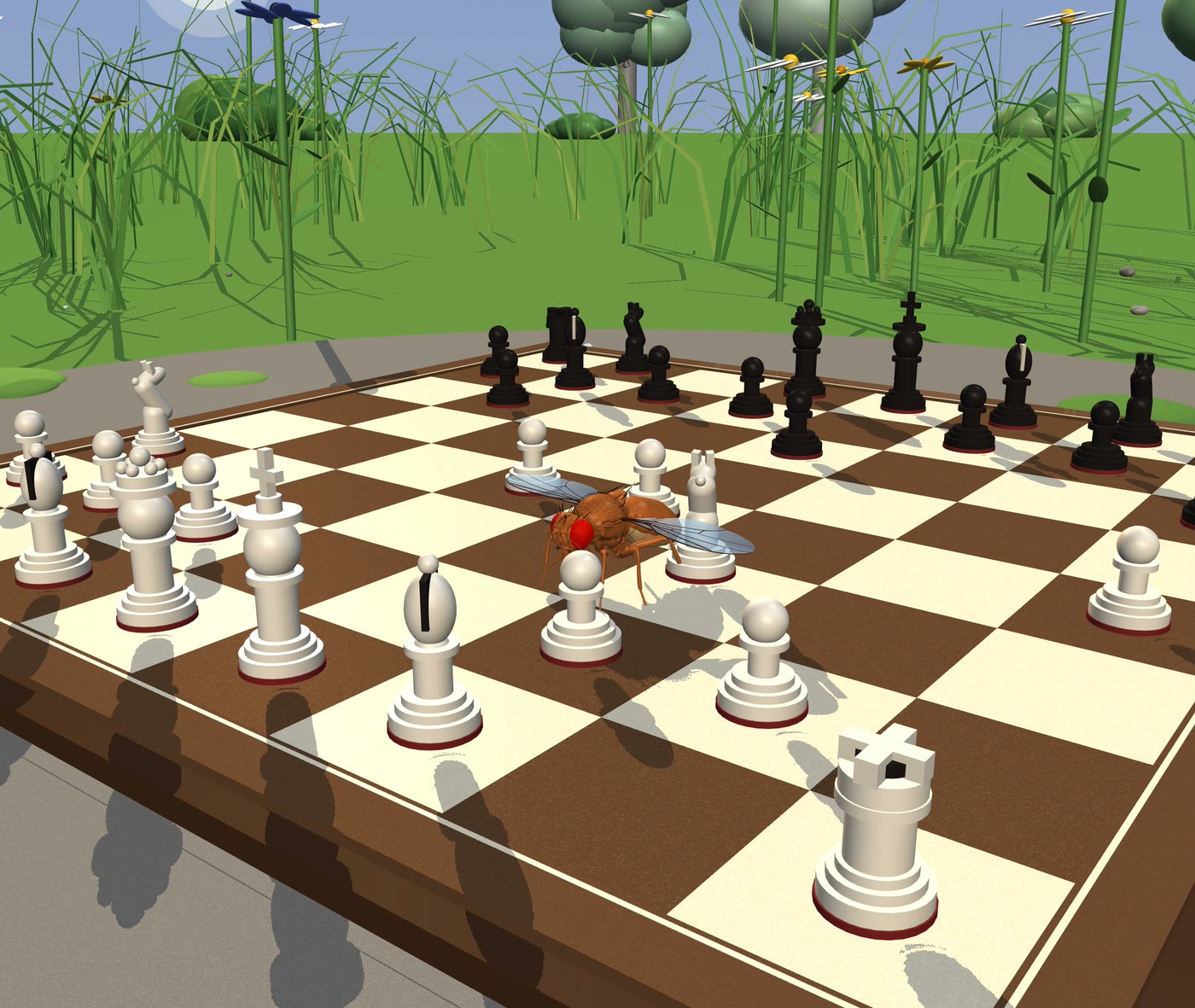
Against the Elo 1320 setting the network won no games and drew five, all because Stockfish repeated positions. A score that close to zero does not support a rating estimate, so I do not give one. In practice the network moves the pieces correctly, protects them some of the time, and has no idea how to finish a game. In the filmed game, Stockfish mates it on move 48.
Figure 7 runs the same network in your browser. It downloads the trained weights once and computes each move on your device, with all 144,209 neurons and 24 ticks per move. The exported weights reproduce the original model's move on all 1,024 positions I tested, and the browser engine matches the exported model on all 64 of its test positions. Appendix A.5 describes how the model was compressed to fit.
Play the network
You play Black. Select a piece, then its destination.Highest-scoring moves
Load the trained network
This downloads 82 MB once and runs every neuron on your device. A move takes one to two seconds on a laptop.
3Results
3.1Where the chess happens
A simulation allows an experiment that is impossible at this scale in a living fly: silence any group of neurons, clamping them to zero at every tick, and measure what is left. I silenced each of 28 groups in turn and measured how often the network chose Stockfish's move on 2,048 positions. These positions are not held out: they come from the same data stream as the first training stage, so most of them were trained on, although with the human's move as the label rather than Stockfish's. The intact network agrees with Stockfish 20.3% of the time. Silencing the descending neurons, which removes everything the readout sees, leaves 5.1%, so I treat the 15.2 points between the two as the part of the network's performance that depends on the board (Figures 8 and 9).
With nothing silenced, the network chooses the same move as Stockfish on 20.3% of 2,048 positions. Select a group to see how that changes.
Silencing the photoreceptors, the optic lobe or the visual projection neurons removes 88 to 99% of that 15.2-point margin. The lamina cells, the Mi, Dm and Tm medulla types and the lobula columnar neurons each remove 35 to 78%. Three visual groups have no measurable effect: the T4 and T5 motion detectors (expected for a board that never moves), the medulla tangential cells and the centrifugal neurons that feed back into the optic lobe.
Silencing the 32,160 intrinsic neurons of the central brain removes about 60% of the margin (20.3% to 11.1%), so the central brain carries much of the signal. None of its best-known structures shows an effect, though: the mushroom body's Kenyon cells and output neurons, the central complex and the lateral horn each change agreement by less than 0.3 points. That null is weaker evidence than it looks. Kenyon cells receive mostly olfactory input, so a null is expected anatomically. The dopaminergic mushroom-body group cannot have any effect at all, because its outgoing connections were removed when the model was built (hatched in Figure 9). And the brain regions that receive the lobula's output were not tested as groups.
Show the data as a table
The measurement itself has a weakness. The descending neurons' activity is of order 10−5, and the readout subtracts a fixed mean and multiplies by fixed scales between 105 and 106. Clamping any group to zero can shift these baselines regardless of what information the group carries, which may be why silencing groups that cannot see the board, such as mechanosensory neurons, still costs about 3 points. Clamping each group to its average activity instead, or refitting the readout after silencing, would separate the two effects; I have not done either. A separate probe in the repository is consistent with the visual picture: a linear readout on a random 1,314-dimensional projection of each population predicts the human move about equally well from the optic lobe (14.2% top-1) and from the descending neurons (14.1%), and slightly worse from the central brain (12.2%).
3.2What training changed
Training changed the network substantially. Using the full effective weights (Appendix A.3), the rank correlation with synapse counts over all 21.27 million connections is $\rho = 0.43$. Most of the change sits in the per-neuron gains: across neurons, the output gains have a median of 0.66 and range from 0.07 to 1.78 between the 1st and 99th percentiles, and the input gains range from 0.46 to 2.43, with a maximum of 63. The per-connection gains moved less, with a median of 0.99, though 41% changed by more than 10%. The project's analysis script reports a correlation of 0.948 between synapse counts and counts multiplied by the per-connection gains alone. That number says nothing: multiplying the counts by random gains with the same spread gives 0.953.
Among the per-connection gains, the inputs turned down hardest come from olfactory receptor neurons, wide-field motion detectors and bristle mechanosensors, none of which carry information about a static board, and 57% of the inputs onto descending neurons were turned down.
Weak connections still matter collectively. If each neuron keeps only the strongest half of its inputs, with no retraining, the network chooses a different move on 41% of 512 positions; keeping the strongest 10% leaves agreement with the full network at 10%. Because every neuron's inputs are normalised, many small connections together make up a large share of its drive.
3.3Learning from its own games
Imitation never tells the network that a move lost material. In the last phase, I let it play 20,477 games against the greedy bot and trained it with PPO, rewarding the result (+1, 0 or −1) plus a shaping term for material balance (Appendix A.3). This phase trained the per-neuron gains, the biases and the move readout, 5.83 million of the model's 27.1 million parameters; the per-connection gains stayed frozen. Training games longer than 200 moves were stopped and scored as draws.
The weights compared below are the run's best checkpoint by its in-training score against the greedy bot, chosen among 92 evaluations, rather than its final weights; that choice favours the greedy matchup. Replaying the matches with identical settings (Figure 10), the score against the random mover fell from 0.666 to 0.624 (−0.042 ± 0.017), against the greedy bot it rose from 0.307 to 0.326 (+0.019 ± 0.019, within noise), and against Stockfish at depth 1 it did not change (−0.009 ± 0.014). Against both weaker opponents, wins and losses fell and draws rose; against the random mover, draws went from 253 to 297 of 400 games.
The material reward is one explanation. A material bonus does no harm to a player that can calculate; for one that cannot, the cheapest way never to lose material is never to commit to anything: shuffle, trade down, hold. Potential-based shaping leaves the optimal policy unchanged in theory,4 but that guarantee says nothing about which policy is easiest to reach with a finite budget. Two other explanations are not ruled out. Scoring 200-move training games as draws also rewards stalling, and the strength of the pull back towards the supervised policy was never varied. Telling them apart needs runs without the material term and without the move cap, over several seeds, compared at their final weights. I have seen a reasonable-looking reward optimised in an unintended way before, while training surgical-robot policies (post forthcoming), which is why I would rather test this than assert it.
4Limitations
The results have no reference point yet. I have not trained the same model on a randomly rewired network with the same number of connections per neuron, with shuffled signs, or as a dense network of the same size. I have also not trained the simpler baselines that would show what the connectome contributes: a readout trained on top of the frozen, untrained brain, or a model reading the photoreceptor encoding directly. Networks trained to predict human moves at a given rating6 give a further comparison for the 23% figure. Until these exist, nothing here shows that the fly's wiring helps.
The evaluation data are not cleanly separated. The silencing, pruning and compression positions come from the same stream as the first training stage. For silencing, the reported agreements were therefore measured largely on training positions. For pruning and compression, which compare two versions of the same network with each other, the overlap matters less.
Match results did not reproduce between runs with the same settings. Against the greedy bot, an earlier 200-game match scored 0.24 (95% interval 0.21–0.28), against 0.31 (0.28–0.34) in the 400-game replay; against Stockfish at depth 1, an earlier match drew 15 of 200 games against 20 in the replay. The earlier matches took over two hours and appear to have run on a laptop CPU, while the replays took minutes on a rented GPU. Given how strongly the readout amplifies tiny differences, numerical differences between the two are a plausible cause, but I have not tested it by replaying the same games on both.
Other irregularities: the supervised weights (step 11,600) were recovered by hand from a checkpoint corrupted when the compute budget ended mid-write, and the later step-12,200 weights were not recovered; the evaluation during reinforcement learning allowed repeated positions, so Figure 10 uses the replay rather than training-time scores; and every configuration was trained once. The model itself is simple: graded rate units with one time constant rather than spiking cells, no modulatory signalling and no gap junctions, and an eye that sees the pieces and the side to move but not castling rights or en passant.
6Next steps
The next experiments, cheapest first: the readout-only and direct-encoding baselines; the rewired, sign-shuffled and dense controls; the silencing experiment repeated on positions from games never used in training, clamping each group to its average activity; and reinforcement learning without the material term or the move cap, over several seeds. If the connectome then beats its rewired versions, the question I most want to answer is whether the circuits it uses resemble the ones a real fly uses to see.
The code, trained weights and an interactive 3D atlas of the brain are on GitHub, and any UCI chess program can load the engine.
ATechnical details
A.1Model
Each neuron $i$ has a graded rate $r_i$, set to zero at the start of every move and updated every tick by
where $n_{ij}$ is the synapse count from $j$ to $i$, $\sigma_j \in \{+1, -1\}$ is the presynaptic sign, $I_i$ is the input current (non-zero only for photoreceptors) and $b_i$ is a bias. I use $\alpha = 1.5$ and $k = \Delta t/\tau = 0.25$, with 5 ms ticks and a 20 ms time constant. The raw signed matrix has a leading eigenvalue of 4,089, dominated by the optic lobe's columnar loops, and any single global scale that keeps it stable starves the central brain's weaker pathways; normalising each row avoids this. At initialisation every row of $|W|$ sums to $\alpha$, so by the Gershgorin circle theorem no eigenvalue of $W$ has modulus above 1.5. Because $\alpha > 1$, this does not guarantee a stable rest state; the saturating $\tanh$ keeps activity bounded, and no run diverged. The bound does not hold after training: the absolute row sums of the trained weights have a median of 0.93, but 45% of rows exceed 1 and the largest is 1,111.
Signs come from the dataset's neurotransmitter predictions: acetylcholine positive (92,375 neurons), glutamate negative (26,874), GABA negative (16,733) and histamine negative (5,902, which include the 4,114 photoreceptors). The outgoing connections of the 774 dopamine, serotonin and octopamine neurons are removed, and the 1,551 neurons without a confident prediction are treated as cholinergic.
A.2Input encoding
Photoreceptors carry no eye coordinates, so each of the right eye's 2,239 placed receptors is assigned to the column of its strongest partner among the cell types that occur exactly once per column (L1–L5, Mi1, Mi4, Mi9, Tm1, Tm2, Tm20 and others). The R1–R6 tracing is partial (380 columns) while R7 and R8 cover about 650 to 700, so the board uses the 645 columns that have both colour receptors. Input currents are $I = \operatorname{artanh}(0.8\,\ell)$ for levels $\ell \in \{0, \tfrac13, \tfrac23, 1\}$, which makes the receptors' rates equally spaced. With a linear drive, the two brightest levels were nearly indistinguishable one synapse downstream.
A.3Training
Supervised training learns a non-negative gain on every connection and an input and output gain for every neuron, so the effective weight is
The 21.27 million $\theta_{ij}$, the per-neuron gains, the biases and the readout heads make 27.1 million parameters, trained by backpropagation through all 24 ticks. No term can change a sign or create a connection, since $\tilde W_{ij} = 0$ wherever $n_{ij} = 0$. A custom autograd function multiplies by a precomputed sparse transpose in the backward pass, so no sparse tensor is ever differentiated. Training used data parallelism over four RTX 5090s, 512 positions per step, 1,500 warm-up steps and 10,700 further steps (191 minutes in total). The move head (4,096 from–to logits plus promotion logits) is unmasked during training, so legality has to be learned. The weights used throughout are from step 11,600: 79.7% legal, 23.0% top-1 and 47.9% top-3 on the stage-2 evaluation set.
The reinforcement-learning phase uses PPO with generalised advantage estimation, an entropy bonus and a KL penalty towards the frozen supervised policy. The critic is a new scalar head on the same descending neurons. The reward for each move is $\beta\,\big(\gamma\,\phi(s') - \phi(s)\big)$, plus the result ($\pm 1$ or $0$) at the end of the game, where $\phi(s) = \tanh(\Delta m(s)/5)$, $\Delta m$ is the network's material balance in pawns, $\phi = 0$ at a finished game, $\beta = 0.5$ weights the shaping and $\gamma = 0.995$ is the discount factor. Training games are stopped at 200 moves and scored as draws. Other settings: GAE $\lambda = 0.95$, clip ratio 0.2, entropy coefficient 0.01, KL coefficient 0.05, 96 games in parallel and 16 moves per game per iteration. The run took 920 iterations, 1.41 million of the network's own moves and 150 minutes on one RTX 4090, at a compute cost of $1.29.
A.4Evaluation
Matches use legal-move masking, the anti-repetition rule, four random opening plies, alternating colours and a 300-move cap scored as a draw. Stockfish runs with UCI_LimitStrength at its floor of 1320 and 50 ms per move, or at search depth 1. Silencing clamps a group to zero at every tick. The pruning test in Section 3.2 keeps the top fraction of each neuron's incoming connections by magnitude and compares moves on 512 positions, without retraining.
A.5Running the model in a browser
The trained checkpoint is a 108 MB file of float32 parameters plus the sparse wiring, which is too large to ship to a web page as it stands. Most of the reduction comes from two steps that change nothing beyond floating-point rounding, and one that does.
The first step is folding. Every factor in the effective weight multiplies, so the per-connection gain, the input and output gains of the two neurons and the normalisation collapse into a single number per connection, $\tilde W_{ij}$ in A.3. This leaves 21.27 million weights, 144,209 biases and the readout. I kept the readout's standardisation of descending-neuron activity separate. The raw activity of those neurons varies over a range of about $10^{-5}$, so folding the standardisation into the readout weights produces very large terms that cancel each other, and those do not survive rounding.
The second step is compressing the wiring. Within each neuron's row of the connection matrix, the column indices are sorted and stored as differences from the previous index, written in a variable-length byte code, so most indices take one or two bytes instead of four. After gzip, the wiring is 31 MB.
The third step is rounding the weights, and it is the only one that can change behaviour. I compared three formats against the original PyTorch model on 1,024 positions, counting how often the compressed network chooses the same move (Table 2).
| Weight format | Same move | Same top three | Size |
|---|---|---|---|
| float16 | 100.0% | 99.9% | 40 MB |
| 8-bit, logarithmic per row | 87.4% | 91.3% | 21 MB* |
| 8-bit, linear per row | 76.5% | 81.2% | 21 MB* |
Half precision reproduces every move. Both 8-bit formats fail, and the reason is the same as in the pruning test of Section 3.2: a neuron's drive is the sum of many small inputs, and 8 bits per row either rounds the small ones to zero (linear) or distorts them enough to shift the descending neurons' output (logarithmic). The readout tolerates 8 bits better, keeping the same move on 98% of positions, but I set 99% as the bar for calling a compressed network the same player, so it also stays at float16 (10 MB).
The page therefore downloads 82 MB once and caches it. A background thread decodes the weights to float32 and runs the same update as A.1 over all 144,209 neurons for 24 ticks per move, which takes about 1.3 seconds on an Apple M4 laptop. On the 64 positions exported as test vectors, the browser engine picks the same move as the exported Python model and the original checkpoint in every case.
References
- Berg et al. (2026). Sexual dimorphism in the complete Drosophila male central nervous system connectome. Cell. Data released under CC-BY by Janelia FlyEM, the Cambridge Drosophila Connectomics Group and Google Research.
- Shiu et al. (2024). A Drosophila computational brain model reveals sensorimotor processing. Nature.
- Lappalainen et al. (2024). Connectome-constrained networks predict neural activity across the fly visual system. Nature.
- Ng, Harada and Russell (1999). Policy invariance under reward transformations: theory and application to reward shaping. ICML.
- Cho, Kang and Kim (2026). A Drosophila whole-connectome network can learn human-designed cognitive tasks. arXiv:2610.10014.
- McIlroy-Young, Sen, Kleinberg and Anderson (2020). Aligning superhuman AI with human behavior: chess as a model system. KDD.